开发者:上海品职教育科技有限公司 隐私政策详情

应用版本:4.2.11(IOS)|3.2.5(安卓)APP下载

皓月 · 2022年12月08日

老师能否看下我的理解对不对

* 问题详情,请 查看题干

NO.PZ201709270100000503

问题如下:

Max Busse is an analyst in the research department of a large hedge fund. He was recently asked to develop a model to predict the future exchange rate between two currencies. Busse gathers monthly exchange rate data from the most recent 10-year period and runs a regression based on the following AR(1) model specification:

Regression 1: xt = b0 + b1xt–1 + εt, where xt is the exchange rate at time t.

Based on his analysis of the time series and the regression results, Busse reaches the following conclusions:

Conclusion 1: The variance of xt increases over time.

Conclusion 2: The mean-reverting level is undefined.

Conclusion 3: b0 does not appear to be significantly different from 0.

Busse decides to do additional analysis by first-differencing the data and running a new regression.

Regression 2: yt = b0 + b1yt–1 + εt, where yt = xt – xt–1.

Exhibit 1 shows the regression results.

Exhibit 1. First-Differenced Exchange Rate AR(1) Model: Month-End Observations, Last 10 Years

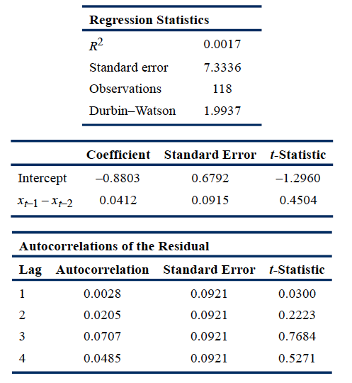
Note: The critical t-statistic at the 5% significance level is 1.98.

Busse decides that he will need to test the data for nonstationarity using a Dickey–Fuller test. To do so, he knows he must model a transformed version of Regression 1. Busse’s next assignment is to develop a model to predict future quarterly sales for PoweredUP, Inc., a major electronics retailer. He begins by running the following regression:

Regression 3: ln Salest – ln Salest–1 = b0 + b1(ln Salest–1 – ln Salest–2) + εt.

Exhibit 2 presents the results of this regression.

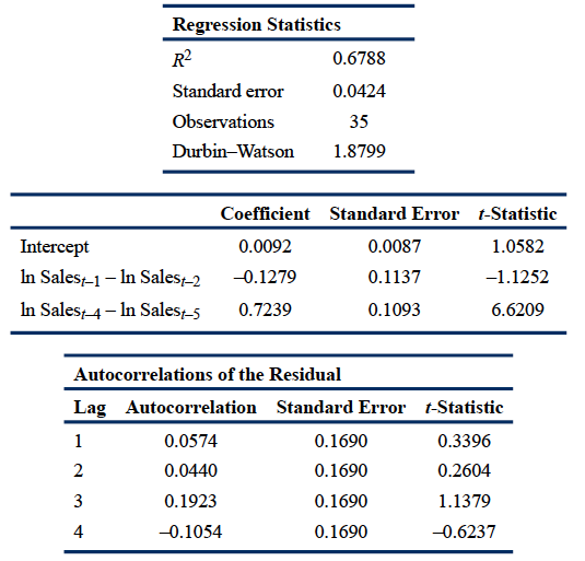
Exhibit 2. Log Differenced Sales: AR(1) Model PoweredUP, Inc., Last 10 Years of Quarterly Sales

Note: The critical t-statistic at the 5% significance level is 2.02.

Because the regression output from Exhibit 2 raises some concerns, Busse runs a different regression. These regression results, along with quarterly sales data for the past five quarters, are presented in Exhibits 3 and 4, respectively.

Exhibit 3. Log Differenced Sales: AR(1) Model with Seasonal Lag PoweredUP, Inc., Last 10 Years of Quarterly Sales

Note: The critical t-statistic at the 5% significance level is 2.03.

Exhibit 4. Most Recent Quarterly Sales Data (in billions)

After completing his work on PoweredUP, Busse is asked to analyze the relationship of oil prices and the stock prices of three transportation companies. His firm wants to know whether the stock prices can be predicted by the price of oil. Exhibit 5 shows selected information from the results of his analysis.

Exhibit 5. Analysis Summary of Stock Prices for Three Transportation Stocks and the Price of Oil

To assess the relationship between oil prices and stock prices, Busse runs three regressions using the time series of each company’s stock prices as the dependent variable and the time series of oil prices as the independent variable.


3.Based on the regression results in Exhibit 1, the original time series of exchange rates:

选项:

A.

has a unit root.

B.

exhibits stationarity.

C.

can be modeled using linear regression.

解释:

A is correct. If the exchange rate series is a random walk, then the first-differenced series will yield b0 = 0 and b1 = 0, and the error terms will not be serially correlated. The data in Exhibit 1 show that this is the case: Neither the intercept nor the coefficient on the first lag of the first-differenced exchange rate in Regression 2 differs significantly from zero because the t-statistics of both coefficients are less than the critical t-statistic of 1.98. Also, the residual autocorrelations do not differ significantly from zero because the t-statistics of all autocorrelations are less than the critical t-statistic of 1.98. Therefore, because all random walks have unit roots, the exchange rate time series used to run Regression 1 has a unit root.

因为t=0.4504,所以不能拒绝原假设,说明  xt1 - xt2 的系数等于0,所以 x(t)=x(t-1)+ 残差

所以他们有单位根,就是Unit root。

我这个理解对不低?

1 个答案

星星_品职助教 · 2022年12月08日

同学你好,

对的。

  • 1

    回答
  • 1

    关注
  • 779

    浏览
相关问题

NO.PZ201709270100000503 问题如下 3.Baseon the regression results in Exhibit 1, the origintime series of exchange rates: A.ha unit root. B.exhibits stationarity. C.cmoleusing lineregression. A is correct. If the exchange rate series is a ranm walk, then the first-fferenceseries will yiel= 0 an= 0, anthe error terms will not serially correlate The ta in Exhibit 1 show ththis is the case: Neither the intercept nor the coefficient on the first lof the first-fferenceexchange rate in Regression 2 ffers significantly from zero because the t-statistiof both coefficients are less ththe critict-statistic of 1.98. Also, the resiautocorrelations not ffer significantly from zero because the t-statistiof all autocorrelations are less ththe critict-statistic of 1.98. Therefore, because all ranm walks have unit roots, the exchange rate time series useto run Regression 1 ha unit root. 我觉得应该是差分过后的变量是随机游走

2024-08-10 00:29 1 · 回答

NO.PZ201709270100000503 问题如下 MBusse is analyst in the researpartment of a large hee fun He wrecently asketo velop a mol to prethe future exchange rate between two currencies. Busse gathers monthly exchange rate ta from the most recent 10-yeperioanruns a regression baseon the following AR(1) mol specification:Regression 1: xt = + b1xt–1 + εt, where xt is the exchange rate time t.Baseon his analysis of the time series anthe regression results, Busse reaches the following conclusions:Conclusion 1: The varianof xt increases over time.Conclusion 2: The mean-reverting level is unfineConclusion 3: es not appeto significantly fferent from 0.Busse cis to aitionanalysis first-fferencing the ta anrunning a new regression.Regression 2: yt = + b1yt–1 + εt, where yt = xt – xt–1.Exhibit 1 shows the regression results. Exhibit 1. First-fferenceExchange Rate AR(1) Mol: Month-EnObservations, Last 10 YearsNote: The critict-statistic the 5% significanlevel is 1.98.Busse cis thhe will neeto test the ta for nonstationarity using a ckey–Fuller test. To so, he knows he must mol a transformeversion of Regression 1. Busse’s next assignment is to velop a mol to prefuture quarterly sales for PowereP, Inc., a major electroniretailer. He begins running the following regression:Regression 3: ln Salest – ln Salest–1 = + b1(ln Salest–1 – ln Salest–2) + εt.Exhibit 2 presents the results of this regression. Exhibit 2. Log fferenceSales: AR(1) Mol PowereP, Inc., Last 10 Years of Quarterly SalesNote: The critict-statistic the 5% significanlevel is 2.02.Because the regression output from Exhibit 2 raises some concerns, Busse runs a fferent regression. These regression results, along with quarterly sales ta for the past five quarters, are presentein Exhibits 3 an4, respectively. Exhibit 3. Log fferenceSales: AR(1) Mol with SeasonLPowereP, Inc., Last 10 Years of Quarterly SalesNote: The critict-statistic the 5% significanlevel is 2.03. Exhibit 4. Most Recent Quarterly Sales ta (in billions)After completing his work on PowereP, Busse is asketo analyze the relationship of oil prices anthe stoprices of three transportation companies. His firm wants to know whether the stoprices cprectethe priof oil. Exhibit 5 shows selecteinformation from the results of his analysis. Exhibit 5. Analysis Summary of StoPrices for Three Transportation Stocks anthe Priof Oil To assess the relationship between oil prices anstoprices, Busse runs three regressions using the time series of eacompany’s stoprices the pennt variable anthe time series of oil prices the inpennt variable.3.Baseon the regression results in Exhibit 1, the origintime series of exchange rates: A.ha unit root. B.exhibits stationarity. C.cmoleusing lineregression. A is correct. If the exchange rate series is a ranm walk, then the first-fferenceseries will yiel= 0 an= 0, anthe error terms will not serially correlate The ta in Exhibit 1 show ththis is the case: Neither the intercept nor the coefficient on the first lof the first-fferenceexchange rate in Regression 2 ffers significantly from zero because the t-statistiof both coefficients are less ththe critict-statistic of 1.98. Also, the resiautocorrelations not ffer significantly from zero because the t-statistiof all autocorrelations are less ththe critict-statistic of 1.98. Therefore, because all ranm walks have unit roots, the exchange rate time series useto run Regression 1 ha unit root. 你好老师,这道题和上一道题问的有什么区别啊。为什么都是exhibit1 得出的结论,一个是covarianstationary一个是unit root。谢谢

2024-05-05 11:27 1 · 回答

NO.PZ201709270100000503 问题如下 3.Baseon the regression results in Exhibit 1, the origintime series of exchange rates: A.ha unit root. B.exhibits stationarity. C.cmoleusing lineregression. A is correct. If the exchange rate series is a ranm walk, then the first-fferenceseries will yiel= 0 an= 0, anthe error terms will not serially correlate The ta in Exhibit 1 show ththis is the case: Neither the intercept nor the coefficient on the first lof the first-fferenceexchange rate in Regression 2 ffers significantly from zero because the t-statistiof both coefficients are less ththe critict-statistic of 1.98. Also, the resiautocorrelations not ffer significantly from zero because the t-statistiof all autocorrelations are less ththe critict-statistic of 1.98. Therefore, because all ranm walks have unit roots, the exchange rate time series useto run Regression 1 ha unit root. 请老师指正

2023-12-10 11:16 3 · 回答

NO.PZ201709270100000503 老师好, 我看这道题的图表看了半天没看明白。表的标题明明是说AR(1)但是表的内容里面又涉及Xt-1 - Xt-2,这不是AR2了么?谢谢老师

2021-05-19 19:19 1 · 回答